
Monte Carlo Simulation for CRE Investments

Monte Carlo simulation is a powerful tool for understanding risk and uncertainty in commercial real estate (CRE) investments. Unlike static models that rely on fixed assumptions, Monte Carlo runs thousands of simulations using probability distributions for variables like rent growth, vacancy rates, and exit cap rates vs. growth rates. This approach provides a range of potential outcomes, helping investors assess risks and probabilities more accurately.
Key takeaways:
- Static models oversimplify: Fixed assumptions often lead to misleading results due to the "Flaw of Averages."
- Monte Carlo uses probability: By assigning distributions (e.g., normal, triangular) to uncertain inputs, it simulates thousands of scenarios.
- More informed decisions: Investors gain insights into risks, expected returns, and the likelihood of hitting specific targets like IRR or NPV.
- Case study: A Cornell study found Monte Carlo predicted an Expected NPV $500,000 higher than static models for a 10-story office building.
- Tools: Excel and platforms like CoreCast simplify running simulations, with CoreCast offering automation and real-time data integration.
Monte Carlo simulation helps CRE investors move beyond rigid assumptions, offering a clearer view of potential outcomes and risks.
How Monte Carlo Simulation Works
Monte Carlo Simulation Process for Commercial Real Estate Investment Analysis
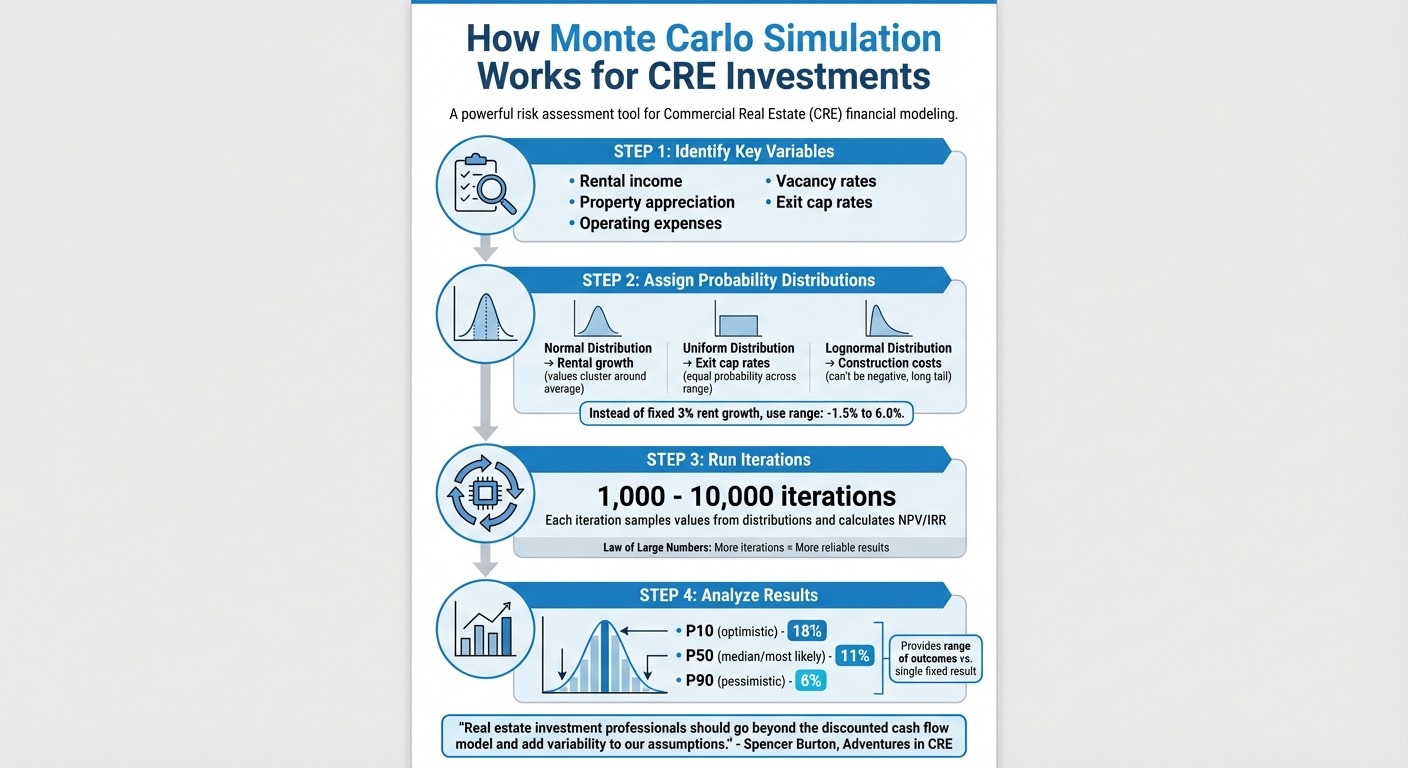
Monte Carlo simulation takes the guesswork out of fixed assumptions by replacing them with probability distributions. Instead of assuming something like "rental growth will be exactly 3%", you define a range - such as –1.5% to 6.0% - and let the model randomly sample values within that range thousands of times. This process generates a spectrum of possible outcomes instead of relying on a single, potentially misleading number [11].
The first step is identifying the variables with the most uncertainty - things like rental income, property appreciation, operating expenses, vacancy rates, and exit cap rates [9]. Then, assign appropriate probability distributions to these variables based on market trends. For example:
- A normal distribution works well for rental growth, as values tend to cluster around a central average (the familiar "bell curve").
- A uniform distribution is ideal for exit cap rates when every value within a range has an equal chance of occurring.
- A lognormal distribution fits construction costs, which can’t be negative and often have a long tail on the higher end [11][6].
Once the distributions are set, run between 1,000 and 10,000 iterations [3]. Each iteration samples a value from each distribution and calculates metrics like net present value (NPV) or internal rate of return (IRR). This can be done in Excel using functions like RAND() or NORM.INV() combined with Data Tables, or with specialized simulation software. Thanks to the Law of Large Numbers, as the number of iterations increases, the results become more reliable and converge toward the true expected value [9].
The results are often displayed as a histogram, showing how frequently different outcomes occur. This approach provides a much clearer picture of uncertainty compared to static models that only offer a single outcome. It directly addresses the unpredictability of market conditions, a key issue in commercial real estate. Spencer Burton, Co-Founder of Adventures in CRE, emphasizes this point:
"Real estate investment professionals should go beyond the discounted cash flow model, an inherently deterministic model, and add variability to our assumptions." [6]
Probability Distributions and Iterations Explained
Probability distributions are at the heart of this method, as they define how uncertainty is represented. For example, in U.S. commercial real estate, historical data shows that property appreciation exceeds 10% in a year only about 7.7% of the time, while it decreases between 0% and 5% roughly 34.6% of the time [10]. A normal distribution captures this tendency for values to cluster near the average. The "68-95-99.7 rule" explains that about 68% of values fall within one standard deviation of the mean, and 95% within two standard deviations [11].
This method also highlights the non-linear nature of real estate returns. Factors like compounding rental growth, leverage, and the interplay between variables mean that the average of all possible outcomes often differs from the outcome calculated using average inputs [1]. As Sarah Lee puts it:
"The Monte Carlo method is based on the principle of generating random samples from a probability distribution and using them to approximate the solution to a mathematical problem." [9]
This foundational understanding makes it possible to apply Monte Carlo simulations effectively to real estate investment scenarios.
Applying Monte Carlo to Real Estate Investments
When applying Monte Carlo simulation to real estate, the key is to replace every uncertain assumption in your discounted cash flow model with a probability distribution. The simulation then runs through every combination of these variables, generating a range of potential NPVs or IRRs.
The resulting distribution can be analyzed using percentiles. For instance, the P50 (median) represents the most likely outcome, while the P10 and P90 show more optimistic and pessimistic scenarios [3]. This allows investors to evaluate both downside risks and upside potential.
Another critical factor is accounting for correlations between variables. For example, if interest rates rise, exit cap rates typically increase as well. Ignoring these relationships could lead to unrealistic scenarios, such as interest rates spiking while yields remain unchanged [3]. Advanced simulations incorporate these correlations, producing results that better reflect real-world market behavior. The outcome is a tool that not only highlights what could happen but also shows how likely each scenario is, helping investors make more informed decisions.
sbb-itb-99d029f
Applications in Commercial Real Estate Investments
Monte Carlo simulation shifts the focus from rigid assumptions to probability distributions, offering a clearer view of risks and opportunities. By applying this framework, investors can better understand variables like cash flow, discount rates, and return projections. Let’s explore how these concepts influence specific aspects of commercial real estate (CRE) investments.
Modeling Cash Flow Uncertainty
Predicting cash flows is rarely straightforward. Traditional discounted cash flow analysis often relies on fixed assumptions, but Monte Carlo simulation introduces probability distributions to key factors like rent growth, vacancy rates, renewal probabilities, operating costs, and capital expenditures [12]. For example, instead of locking in a fixed 3% annual rent increase, simulations might explore variations ranging from –1.5% to 6.0% across thousands of scenarios [11]. Advanced techniques, like Random Walk models, even account for momentum by making each year’s growth dependent on the previous year [12]. These simulations compile countless cash flow outcomes into a probability distribution, giving investors a clearer picture of potential results and their likelihood.
One standout insight is the importance of terminal value, which can account for 75% to 80% of a property’s total discounted cash flow (DCF) valuation [4]. Even small errors - like overestimating rental growth by 1% - can significantly impact long-term projections. To manage this, many investors build in a 5% to 10% buffer to account for uncertainty [4]. As Wall Street Prep explains:
"The DCF output should be viewed as an 'estimation' of a company's value rather than a 'precise calculation' of how much a company is worth." [4]
Evaluating Discount Rate Changes
Discount rates, which reflect factors like interest rates, inflation, credit spreads, and risk premiums, are another critical variable. While traditional DCF models treat the discount rate as fixed, Monte Carlo simulation models it as a range, capturing how valuation reacts to economic changes. For instance, a 200-basis-point change in the discount rate (e.g., from 10% to 12%) can lead to a 27% swing in property value [4]. In the U.S., discount rates for unleveraged CRE investments generally fall between 6% and 12% [9][4].
This method also highlights uneven risks. As Tatchada Supakornpichan, Head of Valuation & Advisory at Cushman & Wakefield, explains:
"The discount rate is the rate of return that an investor expects to receive from investing in a particular asset, taking into account the risk and opportunity of the investment." [8]
Monte Carlo simulation lays out the full range of potential outcomes, making it easier to understand valuation risks tied to discount rate changes.
Projecting IRR and NPV Distributions
Monte Carlo simulation also enhances the analysis of key return metrics like IRR (Internal Rate of Return) and NPV (Net Present Value). By generating distributions for these metrics, it provides a more nuanced view of potential outcomes, often expressed through percentiles such as P10, P50, and P90 [3]. For example, a P90 value suggests a 90% chance of achieving a result better than that figure, which is particularly useful for assessing downside risk.
This approach accounts for the interplay of multiple uncertainties - such as rent growth, vacancy rates, and exit cap rates - offering a depth that basic sensitivity analyses can’t match. As LoopNet points out:
"Saying 'we expect 11% returns' provides false precision. Saying 'we expect P50 returns of 11%, with P10 at 18% and P90 at 6%' communicates both the opportunity and the risk honestly." [3]
These probability distributions help investors pinpoint the highest price they can justify paying for a property, ensuring the NPV remains positive under various scenarios. This method provides a more informed and flexible foundation for making investment decisions.
Step-by-Step Implementation Guide
This guide walks you through the process of running a Monte Carlo simulation for commercial real estate investments. The goal is to pinpoint key variables, assign appropriate probability ranges, and interpret the results effectively.
Setting Up Input Variables and Distributions
Start by identifying the variables that have the biggest impact on your investment returns. These typically include rent growth rates, vacancy rates, operating expense growth, capital expenditures, exit cap rates, and discount rates. These factors play a crucial role in determining metrics like Net Present Value (NPV) and Internal Rate of Return (IRR).
Once you’ve identified these variables, the next step is assigning probability distributions:
- Normal distributions are great for symmetrical variables like rental income, where values cluster around an average.
- Lognormal distributions work well for variables that can't go negative, such as construction costs or property appreciation.
- Triangular distributions require only three inputs - minimum, maximum, and most likely value - and are useful when data is scarce.
- Uniform distributions are ideal for assigning equal probabilities across a range, often used for rent growth or exit cap rates.
Here’s a quick reference table for common variables and their suggested distributions:
| Variable Category | Specific Input Variable | Suggested Distribution |
|---|---|---|
| Income | Rent Growth Rate | Uniform or Normal |
| Income | Vacancy Rate | Triangular |
| Expenses | Operating Expense Growth | Uniform |
| Expenses | Capital Expenditures | Lognormal |
| Exit | Exit Cap Rate | Uniform or Triangular |
| Risk | Discount Rate | Normal |
To ensure accuracy, base your inputs on real-world data and market benchmarks. This helps prevent unreliable results caused by poor-quality inputs.
Choosing Simulation Software and Tools
For many professionals, Excel is the go-to tool. It’s equipped with the RAND() function to generate random probabilities and functions like =NORM.INV(RAND(), [mean], [standard deviation]) to create random inputs based on your selected distributions [1]. Excel’s Data Table feature (found under Data > What-If Analysis) can handle up to 1,000 iterations automatically, eliminating the need for complex macros [7].
For larger portfolios or more advanced needs, platforms like CoreCast offer a streamlined alternative. CoreCast automates data updates, integrates collaboration tools, and simplifies reporting. Unlike spreadsheets, which can be prone to errors and version control issues, CoreCast provides real-time updates and built-in workflows, reducing the chance of mistakes and saving time.
Here’s a comparison of Excel versus CoreCast:
| Feature | Spreadsheet Models (Excel) | SaaS Platforms (CoreCast) |
|---|---|---|
| Customization | High / Fully flexible | Standardized templates |
| Data Updates | Manual entry | Automated / Real-time |
| Collaboration | Challenging / Version issues | Built-in / Real-time |
| Error Risk | High (Human error) | Low (Automated workflows) |
| Reporting | Manual / Time-intensive | Automated / Branded |
| Scalability | Limited for large portfolios | High / Handles complexity |
For those just getting started, specialized Monte Carlo templates tailored to commercial real estate are available on a "Pay What You're Able" basis, starting at $0.00 [7][13]. This makes it easy to experiment with simulations before committing to more advanced tools.
Running Simulations and Reading Results
To ensure reliable outcomes, run at least 1,000 iterations [7]. In Excel, you can set up a column for iteration numbers (1 to 1,000) and use the Data Table tool with a blank cell as the "Column Input Cell" to force recalculations for each row [1]. This generates thousands of possible NPV or IRR outcomes based on your probability distributions.
The Expected Value (mean of all iterations) is your primary output, but there’s more to explore:
- Standard deviation gives you a sense of volatility and risk.
- Percentiles, like the 10th percentile (P10), show downside risk - only 10% of outcomes fall below this level.
- Probability of success is calculated by dividing the number of iterations that meet your target return by the total iterations [1].
Visual tools like histograms are invaluable for presenting results. They illustrate the full range of potential outcomes, offering stakeholders a clearer picture than a single average figure. For instance, in one simulation of a 10-story office building, the Monte Carlo method produced an Expected NPV over $500,000 higher than a static Discounted Cash Flow (DCF) model. This difference stems from Jensen's Inequality and the compounding effects of non-linear variables [1].
Lastly, avoid falling into the "Flaw of Averages": the average of many outcomes is not the same as the outcome of average inputs [1]. This is why Monte Carlo simulations are better suited to capturing the complexities of real estate investments compared to static models.
Advantages and Limitations
Monte Carlo simulation offers a deep dive into investment risk, but it comes with its own trade-offs. A major advantage is its ability to overcome the "Flaw of Averages." Static models, which rely on average inputs, often fail to account for the non-linear effects of variables that interact in complex ways. Monte Carlo simulation addresses this by factoring in these dynamics, leading to more accurate NPV predictions and better-informed investment decisions.
Another strength lies in the probabilistic risk metrics it provides. Unlike deterministic models that produce a single outcome, Monte Carlo simulation generates a range of thousands of potential results, complete with detailed measures like standard deviation, percentiles, and the likelihood of hitting specific return targets. This allows investors to calculate metrics such as Value at Risk (VaR), which helps quantify potential losses in worst-case scenarios. While this method significantly enhances risk analysis, its reliability depends heavily on the quality of the data and the expertise of the user.
That said, Monte Carlo simulation has its downsides. Its accuracy is only as good as the data and assumptions it relies on. Poor-quality inputs or limited historical data can lead to misleading results. For example, real estate returns often display "fat tails" and negative skew - such as the NCREIF Property Index, which has a negative skew of -1.45. This means severe downturns happen more often than a standard bell curve would predict. Using a normal distribution in such cases can result in overly optimistic forecasts, highlighting the need for robust data when using this method.
Another limitation is its complexity. Building and interpreting a Monte Carlo model requires a solid understanding of statistical concepts like mean, standard deviation, kurtosis, and percentiles. This can pose challenges for teams without a quantitative background. Additionally, running these simulations takes more time compared to static models, often requiring advanced Excel skills or specialized software to handle the thousands of iterations involved [2].
Monte Carlo vs. Deterministic Analysis
The differences between Monte Carlo simulation and deterministic analysis are summarized in the table below:
| Aspect | Monte Carlo Simulation | Deterministic Analysis |
|---|---|---|
| Accuracy in Uncertainty Handling | High | Low |
| Computational Requirements | Moderate to High | Low |
| Data Input Needs | Extensive | Basic |
| Interpretation Complexity | Moderate to High | Low |
Deterministic analysis is simpler to create and easier to explain to stakeholders. However, it treats uncertainty as an afterthought, relying on fixed scenarios and ignoring the full range of possibilities. Monte Carlo simulation, on the other hand, demands more effort and statistical expertise but provides a much richer and more nuanced view of potential outcomes. Choosing between these approaches depends on the complexity of the investment, the skill set of your team, and your appetite for risk.
Case Study: Office Building Acquisition
Let's dive into how a Monte Carlo simulation can reshape the investment analysis for a 10-story office building. This approach builds directly on the simulation framework discussed earlier but swaps out fixed assumptions - like a 3% annual rent growth or a 9% exit cap rate - for probability distributions. Key variables in this scenario include rental growth rates, operating expense increases, vacancy periods, tenant renewal probabilities, and the terminal cap rate at sale.
In a study comparing static models to simulations, researchers ran 10,000 iterations and found something striking: using probability distributions resulted in an Expected Net Present Value (ENPV) over $500,000 higher than static models, even when average growth assumptions were identical [1]. This difference stems from what’s called the "Flaw of Averages", where static models fail to capture the non-linear effects of compounding growth. As MIT researcher Keith Chin-Kee Leung explained:
"This is a substantial variation and could be the difference between winning a bid or not" [1].
Instead of offering a single Internal Rate of Return (IRR), the simulation produced a full distribution of outcomes. For example, the P50 (median) IRR provided a realistic base case, while the P10 result indicated only a 10% chance of exceeding an optimistic return, and the P90 result showed a 90% likelihood of outperforming a pessimistic scenario [3]. This allowed stakeholders to communicate risk more effectively. Instead of saying, "We expect 11% returns", they could present: "We expect P50 returns of 11%, with P10 at 18% and P90 at 6%" [3].
The analysis also accounted for variable correlations to reflect actual market dynamics. For example, interest rates and exit yields were modeled with a positive correlation (0.6 to 0.8), as they typically move in tandem. Conversely, vacancy rates and rental growth had a negative correlation (-0.4 to -0.6), showing that weaker markets often experience higher vacancies and slower rent growth [3]. Tenant renewal risks were modeled using discrete probability scenarios, assigning a 70% chance of renewal versus a 30% chance of a 12-month vacancy with associated leasing costs [3].
A tornado chart highlighted the most influential factors, with exit yield movements dominating terminal value impacts. Tenant renewal probabilities and rental growth followed closely, directing due diligence efforts toward cap rate analysis trends. By running the simulation, analysts could pinpoint the likelihood of achieving their 12% IRR hurdle rate and calculate Value at Risk (VaR) for worst-case scenarios - insights that static models simply can't provide. These results laid the groundwork for more integrated and nuanced investment analysis.
Using Monte Carlo Simulation with CoreCast

CoreCast takes Monte Carlo simulation to a new level by automating processes and integrating analysis into one seamless platform. Traditionally, running Monte Carlo simulations required juggling multiple spreadsheets, dealing with manual updates, and managing inevitable formula errors. CoreCast simplifies this by combining data inputs, scenario modeling, and portfolio analysis in a single system. This eliminates the fragmented workflows and data silos that often slow down traditional methods, turning simulation into a faster, more reliable process.
Setting Up Data Inputs and Scenarios in CoreCast
CoreCast uses AI-powered data extraction to automatically pull property details and lease terms from offering memorandums and scanned operating statements. These are then converted into structured data ready for financial modeling [14]. Instead of manually entering rent rolls and operating expenses, the platform syncs with property management systems and market data providers, ensuring consistent and accurate inputs for simulations [14]. Spencer Vickers highlights the impact of this automation:
"By automating data ingestion and real-time assumption adjustments, AI tools eliminate the need for constant formula fixes and recalculations, saving time and reducing errors." [14]
CoreCast also separates input and calculation modules, allowing users to test variables without altering the underlying financial logic [14]. This setup significantly reduces error rates, bringing them down to less than 0.5%, compared to the 5–10% error rates often seen with manual methods [14].
Using CoreCast's Portfolio Analysis for Investment Decisions
Once simulations are complete, CoreCast compiles the results into a dynamic portfolio dashboard. This dashboard showcases how different probability distributions influence overall portfolio performance [8]. Instead of evaluating assets one by one, users can analyze underwriting outcomes across their entire portfolio, uncovering risks like over-concentration or opportunities for diversification.
CoreCast also offers sensitivity analysis tools that highlight critical variables - such as interest rates and vacancy rates - and connects to real-time market data to keep simulation inputs up-to-date [4][14]. By integrating these simulation insights into portfolio analysis, CoreCast provides investors with the tools they need to make informed, data-driven decisions.
Currently in beta and available at $50 per user per month, CoreCast is already gaining traction in the industry. Its ability to handle complex data analysis and predictive modeling with ease reflects the increasing demand for AI-enabled solutions [14].
Conclusion
Monte Carlo simulation transforms how investors tackle uncertainty in commercial real estate by replacing fixed assumptions with probability distributions that simulate thousands of possible outcomes. Instead of relying on a single "best guess", this method provides a detailed risk profile using metrics like P10, P50, and P90, which highlight the likelihood of achieving target returns [3]. It effectively addresses the "Flaw of Averages", where traditional static models fail to capture complexities like compounding rental growth [1].
One of its key advantages is the ability to model correlations between variables and measure downside risk through tools like Value at Risk (VaR). That said, the quality of the simulation's results hinges entirely on the accuracy of the input data. As Real Estate Simpleton aptly puts it:
"Monte Carlo simulation can give thousands of potential outcomes based on variable assumptions... Simulations will not replace the good instincts that are needed in real estate, but can enhance decision making with more information." [5]
Technological advancements have made these simulations more accessible and efficient. Platforms like CoreCast now automate data input and reduce error rates to under 0.5%, a significant improvement over the 5–10% error rates common with manual processes [14]. With 72% of investors already using or planning to adopt AI-powered tools [14], the hurdles to implementing sophisticated probabilistic models have greatly diminished. CoreCast, for instance, integrates underwriting, portfolio analysis, and stakeholder reporting into one streamlined platform, eliminating the fragmented workflows that once made Monte Carlo simulation challenging for smaller firms.
In today’s volatile markets - where something as small as a 1% rise in interest rates can hike mortgage payments by roughly 10% [8] - Monte Carlo simulation offers clear, actionable insights. By automating complex modeling, investors can shift their focus from tedious spreadsheet tasks to making informed, strategic decisions.
FAQs
Which assumptions should I model as distributions first?
When building your analysis, begin by addressing assumptions linked to uncertain factors such as rental growth rates, operating expenses, and other key variables that shape cash flows and valuations. By modeling these variables as probability distributions, you can leverage Monte Carlo simulations to evaluate a wide spectrum of possible outcomes and their corresponding risks. Prioritize the inputs that have the most significant influence on your investment analysis to ensure your findings are as accurate and insightful as possible.
How many iterations are needed for reliable results?
When using Monte Carlo simulations for CRE investments, the number of iterations you need depends on how complex your model is and how precise you want the results to be. Generally, running 1,000 to 10,000 iterations is a good starting point to cover a wide range of possible outcomes. If your model is more intricate or requires greater accuracy, increasing the number of iterations can help improve the reliability and statistical strength of the results.
How do I add correlations (like rates vs. exit caps) in my model?
To incorporate relationships like rates versus exit caps into your Monte Carlo simulation for commercial real estate (CRE) investments, start with a correlation matrix to define how the variables interact. Generate random inputs independently, then use a technique like Cholesky decomposition to introduce the desired correlations. This approach ensures that simulated variables, such as interest rates and exit caps, reflect actual market dynamics, making your analysis more aligned with real-world scenarios.